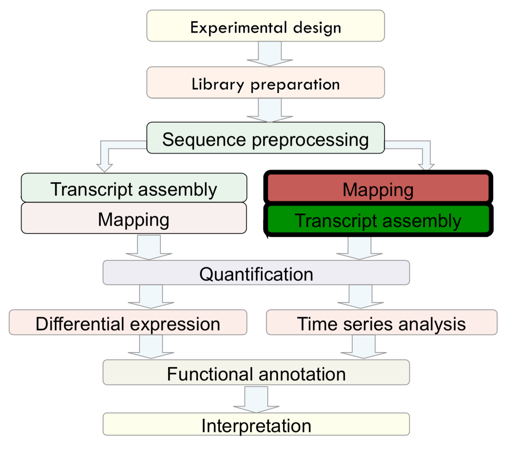
RNA-seq analysis

Runhang / 2019-12-31

今天是二零一九年的最后一天，留学时光匆匆而过，研究生生涯已经过去四分之一。在这里，我把这个学期学了的转录组测序方法总结了一下，放在这里供同行参考讨论。

Introduction

The present study is to trace pluripotency of human early embryos and embryonic stem cells by single cell RNA-seq. To this end, 4-cell embryo and Oocyte cells of human were dissociated into single cell isolation then the cDNAs library were prepared and sequenced on Illumina HiSeq2000 platform.
More than 30 million reads were generated in each single cell sample.
Three biological replicates for each cell type.

Quality Control

After sequencing, we will have fastq file. The first thing we will do is check the quality of the sequence results.

Tool: fastqc (0.11.7)
Script: (Run the bash file in hipergator)

#!/bin/bash
#SBATCH --job-name=fastqc
#SBATCH --time=01:00:00
#SBATCH --mail-user=r.shu@ufl.edu
#SBATCH --mail-type=ALL
#SBATCH --output=fastqc.log
#SBATCH --error=fastqc.err
#SBATCH --nodes=1
#SBATCH --ntasks=1
#SBATCH --mem=20gb.   
#(Note: The command above is typically what we need include in a bash file, 
#in which you tell how many memories, how much time you request)

module load fastqc
fastqc ENCFF000ESM.fastq
fastqc ENCFF000ESS.fastq

Results
Once completed, we will get html files containing basic info of the fastq file such as total reads, GC content, sequence length, and most importantly the per base sequence quality (see the figure below)

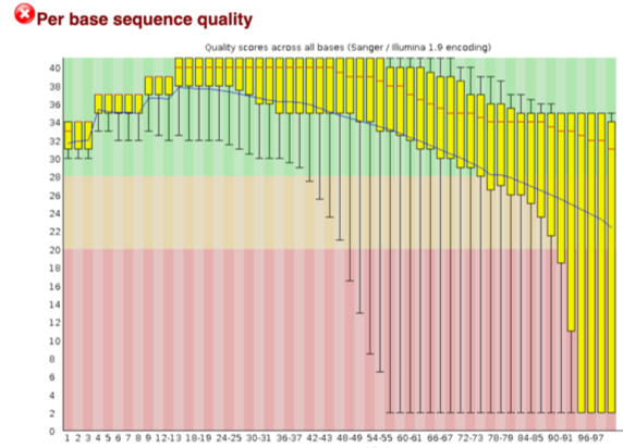
An acceptable sequencing result should have at least 20 quality score (0.01 error rate) across all bases. Score 30 stand for 0.001 error rate. When it is near the end of the reads, the quality score is below 20, so the following Trim and Filter steps are required.

Trim & Filter
Tool: fastxtoolkit
cutadapt (process both pairs at the same time, which is better for paired-end data)
Script:
module load fastxtoolkit/0.0.14
fastqqualityfilter -i ENCFF000ESM.fastq -q 20 -p 50 -o ENCFF000ESM.filtered.fastq
fastqqualityfilter -i ENCFF000ESS.fastq -q 20 -p 50 -o ENCFF000ESS.filtered.fastq
fastqc ENCFF000ESM.filtered2.fastq
fastqc ENCFF000ESS.filtered2.fastq #get rid of reads for which 50% of the bases have quality lower that 20 fastqqualitytrimmer -i ENCFF000ESM.filtered.fastq -t 25 -l 50 -o ENCFFOOOESM.f.t.fastq fastqqualitytrimmer -i ENCFF000ESS.filtered.fastq -t 25 -l 50 -o ENCFFOOOESS.f.t.fastq #trim from the 3’ end until the quality score reach 25 and then remove reads that are shorter than 50 after trimming
Then we run fastqc check the quality again

An alternative of fastx_toolkit is cutadapt
module load cutadapt
cutadapt -a AGATCGGAAGAGCACACGTCTGAACTCCAGTCAC
-AAGATCGGAAGAGCGTCGTGTAGGGAAAGAGTGTAGATCTCGGTGGTCGCCGTATCATT - -quality-base=64 -q 20 -m 50 -o ENCFF000ESM.cutadapt.fastq -p ENCFF000ESS.cutadapt.fastq ENCFF000ESM.fastq ENCFF000ESS.fastq
fastqc ENCFF000ESM.cutadapt.fastq
fastqc ENCFF000ESS.cutadapt.fastq

Mapping
After sequence preprocessing, we can align sequencing reads to a reference (if we have reference genome). There are 2 options in term of mapping:

Mapping against the Genome (Good option is only gene level quantification is needed)
Mapping against the Transcriptome (Good option with will annotated species)

Tools: Bowtie2 and TopHat
Script:
module load bowtie2

build the spliced index of human genome hg38.fa file in bowtie2

bowtie2-build /ufrc/mcb4325/share/Week12/hg38.fa hg38 use the index built by bowtie2 for mapping
module load tophat
tophat2 –no-coverage-search hg38 ENCFFOOOESM.f.t.fastq ENCFFOOOESS.f.t.fastq
Results:
We will get a “Tophatresults” fold with acceptedhits.bam file in it.
BAM file is a compression format of SAM file - Binary file; Save disk (80% compression); Indexed for efficient data access; - Easy to interconvert using SAMtools - BAM to SAM
samtools view -h name.bam > name.sam - Sort BAM file by chromosomal coordinates
samtools sort name.bam name.sorted

Quantification

Method 1
As we already have the bam file, there is no need to assemble the reads for quantification. Again, we mapped the reads based on reference genome. Now, we quantify the reads based on reference genome (Homosapiens.GRCh28.86.OK.gtf file).

Tool: htseq; samtools
Scripts:
module load samtools
module load htseq
samtools sort -n ../Tophatresults/Embryo1/acceptedhits.bam -o sortedE1.bam
htseq-count -f bam -s no -i geneid sortedE1.bam ./Homosapiens.GRCh38.86.OK.gtf > htseqcount_E1.txt

Results:
The result file is a txt file with Ensembl gene_id (such as ENSG0000.) and the number of counts.

Method 2 (Assembly and then quantify)
We can assemble the read based on reference genome with cufflinks and then we get both genes and isoform(transcripts) FPKM file.
FPKM stands for Fragments Per Kilobase of transcript per Million mapped reads, which normalize the basis of gene length because the longer a read is the more count it will have. So, I think this method is better than read count.

Assembly
Tool: cufflinks
Script:
module load cufflinks
cufflinks –library-type fr-firststrand -o /home/r.shu/norefassembly /home/r.shu/tophatout/acceptedhits.bam
#tophat mapped bam file was assembled without reference
OR…
cufflinks -g ../hg38.gtf –library-type fr-firststrand -o /home/r.shu/gassembly /home/r.shu/tophatout/acceptedhits.bam
#tophat mapped bam file was assmebled by GFT reference guide
#hg38 gtf file is reference genome file
OR…
cufflinks -G ./hg38.gtf –library-type fr-firststrand -o /home/r.shu/Gassembly /home/r.shu/tophatout/acceptedhits.bam
#tophat mapped bam file was assembled based on transcripts existing in GFT file

Results: We can get gene.fpkmtracking and isoforms.fpkmtracking files, and importantly, we get transcripts.gtf file which can be visualized in IGV software.
The tacking.gtf files contain quantification info that we can read in R.

De novo Assembly, then mapping and quantifying
For study organisms that are not well annotated genome, we may want to use some algorithm to assemble the raw reads together without any reference.
Tool: trinity; gmap
Script:
module load trinity
Trinity –seqType fq –maxmemory 5G –left /ufrc/mcb4325/share/Week12/UHLEN1T110R1.fastq –right /ufrc/mcb4325/share/Week12/UHLEN1T110R2.fastq –CPU 6
# we get Trinity.fasta file from this process
# If we have reference genome, we can map the trinity assembly result using GMAP
module load gmap
gmapbuild -D . -d hg38.GMAP /ufrc/mcb4325/share/Week12/hg38.fa
# -D means the directory, -d means the name of the file
cd trinityoutdir
gmap -n 1 -t 8 -f 2 -D ../ -d hg38.GMAP Trinity.fasta > Trinity.gff
# -f 2 indicate output format and produce .gff file
awk ‘{if ($3 == “exon”) print $0}’ Trinity.gff > Trinity.exon.gff

Note: De nova transcriptome assembly has higher sensitivity to discover novel transcripts and trans-spliced transcripts BUT not as sensitive as reference-based assembly to discover low-abundance transcripts.

Differential expression analysis
We then move to R for statistics analysis. By now, we have quantified the number of each exon or gene. Also, get the gene length and GC content txt file from Ensembl to check the bias
mycounts_t = read.delim(“CountData.txt”)

dim(mycounts)
head(mycounts)

mylengtht = read.delim(“genetranscript_length.txt” ,as.is = TRUE)
dim(mylength)
head(mylength)

myGCt = read.delim(“geneGC_content.txt”, as.is = TRUE)
dim(myGC)
head(myGC)

Experimental design

myfactorst = data.frame(“treat” = substr(colnames(mycountst), start = 1, stop = 1), “time” = substr(colnames(mycountst), start = 3, stop = 3), “cond” = substr(colnames(mycountst), start = 1, stop = 3))
rownames(myfactorst) = colnames(mycounts)
head(myfactorst)
myfactors_t

Loading R libraries to be used

if (!requireNamespace(“BiocManager”, quietly = TRUE)) install.packages(“BiocManager”)
BiocManager::install(“EDASeq”, version = “3.8”)
BiocManager::install(“NOISeq”, version = “3.8”)
library(NOISeq)
library(EDASeq)

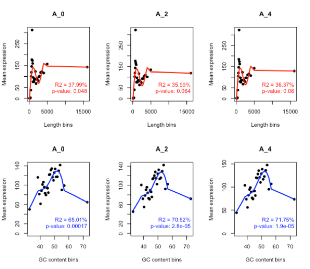
*Note: As the read length and GC content bias is common in Illumina sequencing, where longer read get more counts (FPKM) and low GC content get lower counts. *

BIAS ANALYSIS with NOISeq ########################

Preparing data for NOISeq package

mydata = NOISeq::readData(data = mycounts, factors = myfactors, gc = myGC, length = mylength)

Length bias

mylengthbias = dat(mydata, factor = “cond”, norm = FALSE, type = “lengthbias”)
par(mfrow = c(1,2))
explo.plot(mylengthbias, samples = 1)
explo.plot(mylengthbias, samples = 1:8)

GC content bias

myGCbias = dat(mydata, factor = “cond”, norm = FALSE, type = “GCbias”)
par(mfrow = c(1,2))
explo.plot(myGCbias, samples = 1)
explo.plot(myGCbias, samples = 1:8)

RNA composition

mycomp = dat(mydata, norm = FALSE, type = “cd”) par(mfrow = c(1,2)) explo.plot(mycomp, samples = 1:12) explo.plot(mycomp, samples = 13:24)

NORMALIZATION

First we remove genes with 0 counts in all samples

mycountst = mycountst[rowSums(mycounts_t) > 0, ]

Discarding genes without GC content information

genesWithGCt = intersect(rownames(mycountst), myGCt[,“gene”]) myGCt = myGCt[myGCt[,“gene”] %in% genesWithGCt,] rownames(myGCt) = myGCt[,“gene”] mycountst = mycountst[myGCt[,“gene”],]

head(mycountst) head(myfactorst)

Preparing data for EDASeq package

edadata = newSeqExpressionSet(counts=as.matrix(mycountst), featureData=myGCt[,2, drop = FALSE], phenoData=myfactors_t[,“cond”, drop = FALSE])

Correcting GC content bias with EDASeq package: loess method

edadata <- withinLaneNormalization(edadata,“GCcontent”, which=“full”) mynormdata = edadata@assayData$normalizedCounts

Applying TMM normalization (between-samples) with NOISeq package

mynormdata = tmm(mynormdata) head(mynormdata)

Checking the normalization results

More uniform distributions by TMM

par(mfrow = c(1,2)) boxplot(log(as.matrix(mycounts+1)) ~ col(mycounts), main = “Before normalization”) boxplot(log(mynormdata+1) ~ col(mynormdata), main = “After normalization”)

GC bias memoved

mydata.norm = NOISeq::readData(data = mynormdata, factors = myfactors, gc = myGC, length = mylength) myGCbias = dat(mydata.norm, factor = “cond”, norm = TRUE, type = “GCbias”) par(mfrow = c(1,2)) explo.plot(myGCbias, samples = 1) explo.plot(myGCbias, samples = 1:8)

Loading R libraries to be used

if (!requireNamespace(“BiocManager”, quietly = TRUE)) install.packages(“BiocManager”) BiocManager::install(“DESeq2”) BiocManager::install(“limma”) BiocManager::install(“maSigPro”) BiocManager::install(“statmod”) BiocManager::install(“edgeR”)

library(NOISeq) library(edgeR) library(DESeq2) library(limma) library(maSigPro) library(“edgeR”)

edgeR to profile the differentially expressed genes

############################

cond2compare = colnames(mycounts)[c(grep(“B0”, colnames(mycounts)), grep(“B6”, colnames(mycounts)))] cond2compare mygroups = rep(c(“B0”, “B6”), each = 3) mygroups

edgeR

myedgeR = DGEList(counts = mycounts[,cond2compare], group = mygroups)
myedgeR = calcNormFactors(myedgeR)

myedgeR = estimateCommonDisp(myedgeR)
myedgeR = estimateTagwiseDisp(myedgeR, trend = “movingave”)
myedgeR = exactTest(myedgeR)
names(myedgeR)
head(myedgeR$table)
topTags(myedgeR)
myedgeRdecide = decideTestsDGE(myedgeR, adjust.method = “BH”, p.value = 0.05, lfc = 0)
summary(myedgeRdecide) #Apart from edgeR, we can also use DESeq2 and NOIseq.

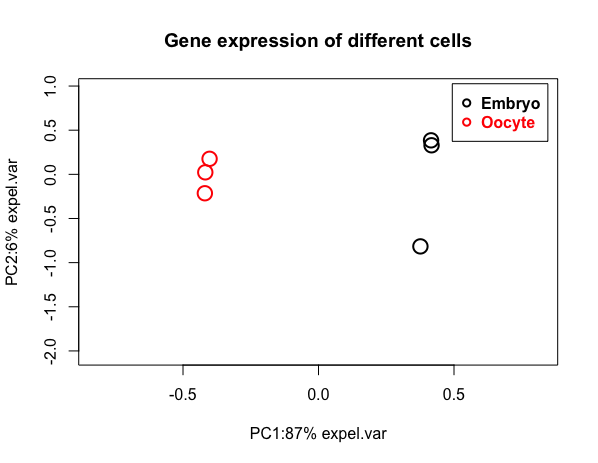
Reduce the dimension by PCA plot

Though there are thousands of variables(gene expression) in each treatments, with Principal coordinate analysis plot, we can appreciate the similarity between two or more samples.

Script
PCA<-princomp(normal_data,cor = TRUE)

create my PCA plot function

myPCAplot<- function(x, main,col=rep(c(1:6),each=3)) {
t.var<-cumsum(x$sdev^2^/sum(x$sdev^2^))
var.PC1<-round(t.var[1]100)
var.PC2<-round((t.var[2]-t.var[1])100)
plot(P[,1],P[,2],
main = main,
col=col,
cex=2, lwd=2,
xlim=c(min(P[,1])-0.1,max(P[,1])+0.1) ,
ylim=range(P[,2])*1.3,
xlab= paste(“PC1:“,var.PC1,”% expel.var”, sep = “”),
ylab=paste(“PC2:“,var.PC2,”% expel.var”, sep = “”) )
legend(x=0.55,y=0.6,legend=c(“Embryo”,“Oocyte”),
col =c(1:2),cex=1,bty=“o”,pch=1,text.font = 2,text.col = c(1:4),
pt.cex = 1,pt.lwd = 2,xjust = 0.5,yjust = 0.5) }
apply the function I created and input the PCA dataset
myPCAplot(PCA, main= (“Gene expression of different cells”))

positive values on x axis indicate the data is not centered

mydata.c<-t(apply(normaldata, 1, scale, scale=FALSE))
colnames(mydata.c)<-colnames(normaldata)
PCA.c<-princomp(mydata.c,cor=TRUE)
myPCAplot(PCA.c, main=“Drug doses effect on genes expression of mice”)

Top10<- sort(abs(PCA.c$scores[,1]), decreasing= TRUE)[1:10]

Use scores ranking in PCA analysis as determinants for the top 10 differentially expressed genes.

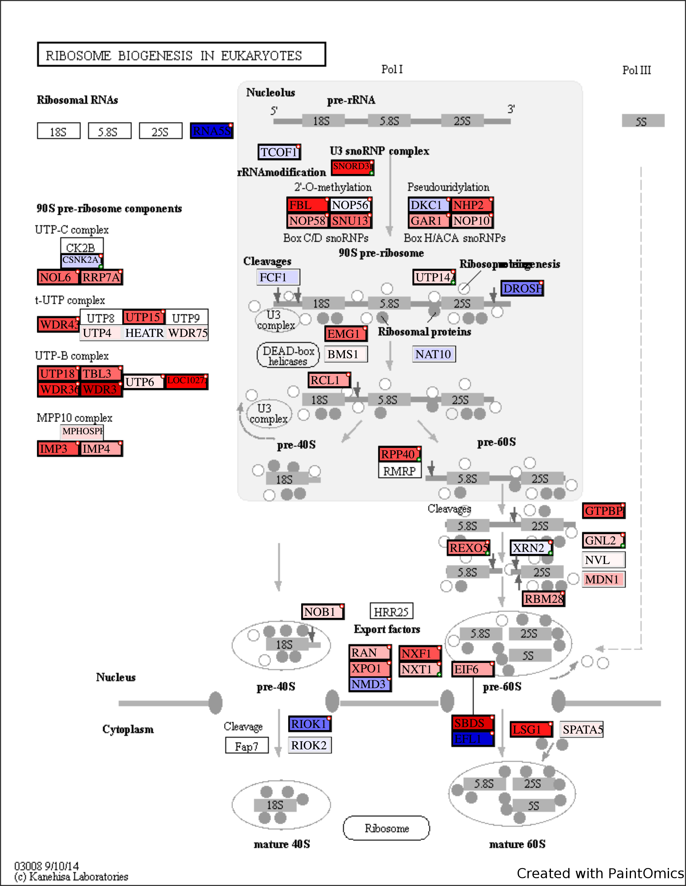
Enrichment and Pathway Analysis
Tool: PaintOmics3

source(“http://bioconductor.org/biocLite.R")
biocLite(“NOISeq”)
biocLite(“goseq”)
biocLite(“goglm”)
library(NOISeq)
library(goseq)

setwd(“/Users/darson/Desktop/Genomics in R/Week 16/DataWeek16”)

NOISeq analysis

data <- read.delim(“Differentiation.txt”, as.is = TRUE, header = TRUE, row.names = 1)

normalized data

mygroups = rep(c(“P”, “D”), each = 3)

data.f = filtered.data(data, factor = mygroups, norm = TRUE, cv.cutoff = 200, cpm = 5) #filter low count genes mynoiseqbio = readData(data.f, factors = data.frame(“condi”=mygroups)) mynoiseqbio = noiseqbio(mynoiseqbio, norm = “n”, k = NULL, factor = “condi”, r = 30) mynoiseqbio.deg = degenes(mynoiseqbio, q = 0.99)

mynoiseqbio.deg <- mynoiseqbio.deg[abs(mynoiseqbio.deg[“log2FC”])> 0.3,]

Enrichment analysis

We obtain GO and gene length from Biomart

GOannot <- read.delim(“mmuGO.txt”, as.is = TRUE, header = TRUE)

Obtain gene length

mmuLength <- read.delim(“mmuLength.txt”, as.is = TRUE, header = TRUE)

mmuLength <- tapply(mmuLength[,3],mmuLength[,1], median)

Preparing data for GOseq analysis

mygenes = rownames(data.f) mmuLength = mmuLength[mygenes] NOISeq.DE = as.integer(mygenes %in% rownames(mynoiseqbio.deg)) # logical vector of DE names(NOISeq.DE) = mygenes head (NOISeq.DE,10)

GOseq

mipwf <- nullp(NOISeq.DE, bias.data = mmuLength)
walle <- goseq(pwf = mipwf, gene2cat = GOannot, method = “Wallenius”, repcnt = 2000)
enriched <- walle$category[walle$overrepresentedpvalue< 0.01]
GO.enriched <- GOannot[match(enriched, GOannot[,2]),3] # obtain GO names
head (GO.enriched, 30) # GO results
tail (GO.enriched, 30) # GO results

Prepare data for Paintomics

mynoiseqbio.all = degenes(mynoiseqbio, q = 0)
expr.data <- cbind (name = rownames(mynoiseqbio.all), FC = mynoiseqbio.all[,“log2FC”])
write.table( expr.data, “expr.data.txt”, row.names = F, col.names = T, quote = F, sep = “\t” )
write.table(rownames(mynoiseqbio.deg), “DE.data.txt”, row.names = F, col.names = F, quote = F, sep = “\t” )

Upload expr.data and DE.data.txt files in PaintOmics